Simpson’s Rule Calculator
Simpson’s rule calculator’s main application is to find the approximate area under a graph. It can find the closest value of the area of a definite integral.
This tool is a Simpson ⅓ rule calculator due to the fact that it uses quadratic functions to find approximations.
The graph of the function with the labeled divisions is also displayed along with the answer. Moreover, this graph can be zoomed in and out.
How to use this Simpson’s rule calculator?
This calculator is simple to use. You will have to:
- Enter the function in the required area.
- Input the values of a and b i.e start point and endpoint of the curve for the area.
- Put the n value.
- Click calculate.
- The result will appear on the screen in a fraction of a second.
- Press the clear button to recalculate.
What is Simpson's rule?
Simpson’s Rule is another method to estimate the area of a nonlinear graph like the left and right Riemann’s sum and Midpoints sum.
It is an algorithmic application of the 1-4-1 quadratic approximation which finds the best fitting parabolas instead of rectangles. This approximation can be applied to the signed areas as well.
Derivation of Simpson’s rule: Simpson’s formula
As mentioned before, Simpson's rule originates from the quadratic approximation. So, before heading ahead, let’s review what it means.
1-4-1 approximation:
Divide a graph into equally spaced sample points at the end and the middle let's say of the half-width h.
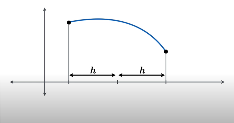
Now, this division can help to find the function values or the y-axis values i.e YL, YC and YR required in the formula. When these four values are used then the area under the quadratic curve that passes through these points can be expressed as
= h/3 (yL + 4yC + yR)
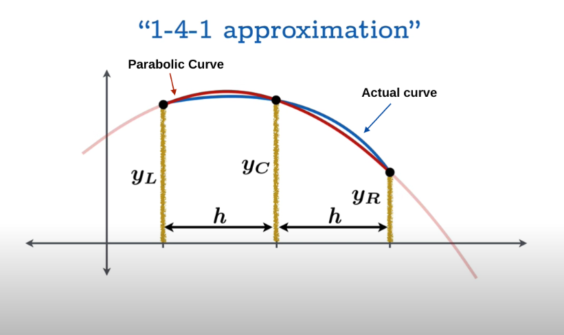
This is approximately equal to the area under the curve as well.
Simpson’s rule:
Now, the example discussed above is a simple and ideal one. Not every curve is sleek and smooth like this. If we apply it on irregular graphs, it will tell an extremely inaccurate value of the area. For example, see this graph below.
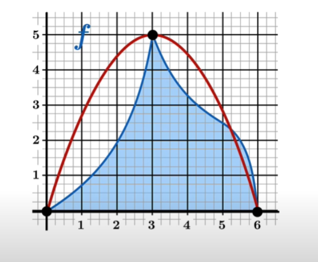
So to find the area under some irregular graph, we cannot apply the quadratic approximation one time. Instead, we divide it into a suitable number of curves so that each curve can give a decent estimation of the parabolic area under it.
For instance, have a look at this graph
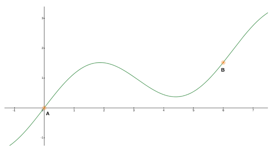
Let's say you are interested in finding the definite integral for this curve between point a and point b.
The goal is to use the approximation repeatedly on this function to get the area estimation. Secondly, we will make subdivisions of equal length to ensure that “half widths” are uniform.
Lastly, Subintervals that we denote with n, have to be in even numbers for the application of the 1-4-1 approximation.
Now that we have gone over the fundamentals, it is time to divide this graph. We will assume a general situation without any defined domain.
Start labeling the endpoint from \(x_0,\:x_1\) and so on to \(\) and \(x_n\).
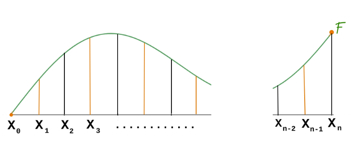
After that, we will let the common half-width be Δx.
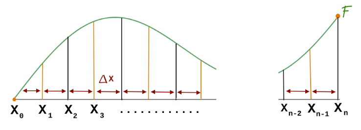
Note: In this graph, black lines represent the divisions of the parabolic curves and the orange lines are subdivisions.
Now, is the time to apply the quadratic approximation. For the first pair of subintervals, we have
\(\frac{Δx}{3}\left(f\left(x_0\right)+4f\left(x_1\right)+f\left(x_2\right)\right)\)
It is explained as half-width divided by 3 into the sum of the left-hand function value, center function value, and right-hand function value.
For the second pair, our contribution is:
\(\frac{Δx}{3}\left(f\left(x_2\right)+4f\left(x_3\right)+f\left(x_4\right)\right)\)
And then the third.
\(\frac{Δx}{3}\left(f\left(x_4\right)+4f\left(x_5\right)+f\left(x_6\right)\right)\)
Now if we add all three expressions, the sum will be:
\(\frac{Δx}{3}\left(f\left(x_0\right)+4f\left(x_1\right)+2f\left(x_2\right)+4f\left(x_3\right)+2f\left(x_4\right)+4f\left(x_5\right)+f\left(x_6\right)\right)\)
The delta x over 3 is taken as common. One can notice that certain values like f(x2) contribute to each other and make 2f(x2). Moreover, there is a certain pattern of coefficients i.e 1,4,2,4,2,4,1.
So going back to the general case, the summed expression will be:
\(\frac{Δx}{3}\left(f\left(x_0\right)+4f\left(x_1\right)+2f\left(x_2\right)+4f\left(x_3\right)+2f\left(x_4\right)+4f\left(x_5\right)+...+f\left(x_n\right)\right)\)
There are pairs of 4 and 2 all over, internally. The first and last single values make a pair. So only the second last value (n-1) is left alone. It means there are odd numbers of values.
This is Simpson's rule.
To find delta x, minus the endpoint from the starting point of the curve and divide by n.
How to apply Simpson’s rule?
The best way to apply Simpson’s rule is to use an online tool like the calculator above. If you don't have access to any tool then read the steps coming up ahead to learn to apply Simpson's rule manually.
If the graph is given, then
- Analyze the graph to divide it into a fair even number of uniform subdivisions to vaguely cover the whole area between points.
- Name the divisions and apply the pattern of the coefficients.
- Multiply the whole thing by delta x over 3.
- Solve.
If the value of n is given, then
- Find the Δx as taught before.
- Use the Δx to make the subdivision. Must be in an odd number!
- Apply the pattern and multiply with Δx/3 as before.
- Solve.
Solved example:
Apply Simpson's rule on the function below and find the error as well.
\(\int _1^4\:\left(x^2+4\right)dx\)
n = 6
Solution:
Step 1: Find Δx.
\(Δx=\frac{b-a}{n}\)
\( Δx=\frac{4-1}{6}\)
\( Δx=0.5\)
Step 2: Divide the intervals [1,4] into n=6 subintervals with the length Δx=0.5.
a = 1, 1.5, 2, 2.5, 3, 3.5, 4
Step 3: Evaluate the function at these endpoints.
f(x0) = f(1) = 12 + 4 = 5
4f(x1) = 4f(1.5) = 4(1.52 + 4) = 25
2f(x2) = 2f(2) = 2(22 + 4) = 16
4f(x3) = 4f(2.5) = 4(2.52 + 4) = 41
2f(x4) = 2f(3) = 2(32 + 4) = 26
4f(x5) = 4f(3.5) = 4(3.52 + 4) = 65
f(x6) = f(4) = 42 + 4 = 20
Step 4: Add these values.
= 5 + 25 + 16 + 41 + 26 + 65 + 20
= 198
Step 5: Multiply with Δx/3.
= 0.5/3 (198)
= 33
Step 6: Find the definite integral.
\(\int _1^4\:\left(x^2+4\right)dx\)
= 33
Step 7: Find the error by subtracting the integral value from the approximation value and also dividing it by the integral value.
= (33 - 33) / 33
= 0%
This is one of those rare cases where integral value and Simpson's rule value are the same.